SpreadSheet Munging Strategies in Python - Small Multiples

Small Multiples

updated : April 14, 2022

This is part of a series of blog posts about extracting data from spreadsheets using Python. It is based on the book written by Duncan Garmonsway, which was written primarily for R users. LInks to the other posts are on the homepage.

Small multiples refer to mini tables embedded in a spreadsheet, or multiple spreadsheets. Ideally, this tables should be lumped into one dataframe for meaningful analysis. The examples below show different scenarios and how we can reshape the data

Case 1 : Small Multiples with all Headers Present for Each Multiple

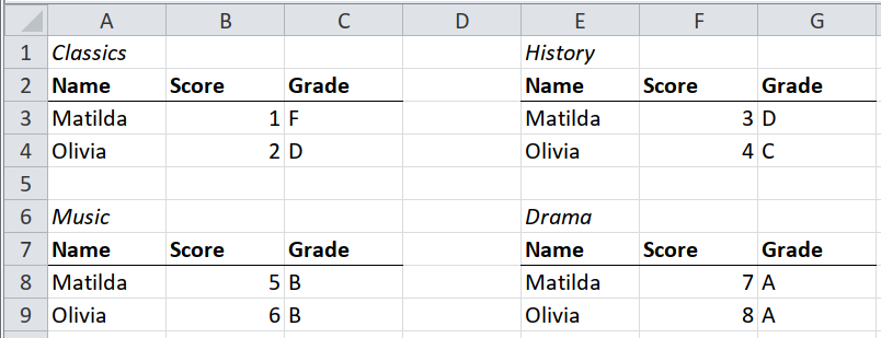
In this spreadsheet, each table is a separate subject. It would be better to aggregate all the subjects and underlying data into one table.

import pandas as pd
import janitor
import numpy as np

excel_file = pd.ExcelFile("Data_files/worked-examples.xlsx", engine='openpyxl')

df = excel_file.parse(sheet_name="small-multiples", header=None)
df

	0	1	2	3	4	5	6
0	Classics	NaN	NaN	NaN	History	NaN	NaN
1	Name	Score	Grade	NaN	Name	Score	Grade
2	Matilda	1	F	NaN	Matilda	3	D
3	Olivia	2	D	NaN	Olivia	4	C
4	NaN	NaN	NaN	NaN	NaN	NaN	NaN
5	Music	NaN	NaN	NaN	Drama	NaN	NaN
6	Name	Score	Grade	NaN	Name	Score	Grade
7	Matilda	5	B	NaN	Matilda	7	A
8	Olivia	6	B	NaN	Olivia	8	A

Observations :

1. There is a completely empty column that splits the tables, and a completely empty row as well. We’ll use the coordinates in our data reshaping

2. For each table, the subject is directly above. We’ll use the empty cells adjacent to it as a criteria to create a subject column

#get the first three columns before the completely null column
before_null = df.iloc[:,:3]
#get the columns after the completely null column
after_null =  df.iloc[:,4:].set_axis([0,1,2],axis=1)

(pd          
.concat((before_null, after_null))
.set_axis(['Name','Score','Grade'],axis=1)
.query('Name != "Name"')
.dropna(subset=['Name'])
.assign(subject = lambda x: np.where(x.Score.isna(), 
                                        x.Name, 
                                        np.nan)
        )
.assign(subject = lambda df: df.subject.ffill())
.dropna()
.reset_index(drop = True)
)

	Name	Score	Grade	subject
0	Matilda	1	F	Classics
1	Olivia	2	D	Classics
2	Matilda	5	B	Music
3	Olivia	6	B	Music
4	Matilda	3	D	History
5	Olivia	4	C	History
6	Matilda	7	A	Drama
7	Olivia	8	A	Drama

The image below illustrates the main concepts of the above code.

Case 2 : Same table in several worksheets/files (using the sheet/file name)

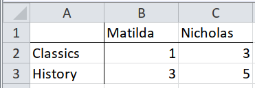
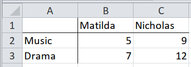
For this case, our data is in different worksheets. We can iterate through each worksheet and combine the dataframes into one.

extract = [excel_file.parse(sheet_name=sheetname, index_col=0) 
           for sheetname in ("humanities", "performance")]

extract

[          Matilda  Nicholas
 Classics        1         3
 History         3         5,
        Matilda  Nicholas
 Music        5         9
 Drama        7        12]

Combine the individual dataframes into one:

(pd
.concat(extract)
.rename_axis(index = 'subject', columns='student')
.stack()
.rename('scores')
.reset_index()
)

	subject	student	scores
0	Classics	Matilda	1
1	Classics	Nicholas	3
2	History	Matilda	3
3	History	Nicholas	5
4	Music	Matilda	5
5	Music	Nicholas	9
6	Drama	Matilda	7
7	Drama	Nicholas	12

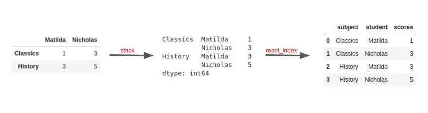
The image below illustrates the core concepts of the above solution:

Case 3 : Same table in several worksheets/files but in different positions

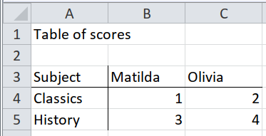
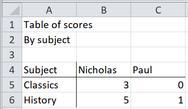
This is similar to Case 2, with the core data been the same. Here we need to pick rows from Subject downwards only, as that is the only relevant data:

extract = {sheetname : excel_file.parse(sheet_name=sheetname, header = None, index_col=0)
                                 .loc['Subject':]
                                 # use the subject row as column names
                                 .pipe(lambda df: df.set_axis(df.loc['Subject'], axis = 1))
                                 .drop(index='Subject')
                                 .rename_axis(index = 'subject', columns = 'student')
           for sheetname in ("female", "male")}

extract

{'female': student  Matilda Olivia
 subject                
 Classics       1      2
 History        3      4,
 'male': student  Nicholas Paul
 subject               
 Classics        3    0
 History         5    1}

Combine the individual dataframes into one:

(pd
.concat(extract, names=['sex'])
.stack()
.rename('scores')
.reset_index()
)

	sex	subject	student	scores
0	female	Classics	Matilda	1
1	female	Classics	Olivia	2
2	female	History	Matilda	3
3	female	History	Olivia	4
4	male	Classics	Nicholas	3
5	male	Classics	Paul	0
6	male	History	Nicholas	5
7	male	History	Paul	1

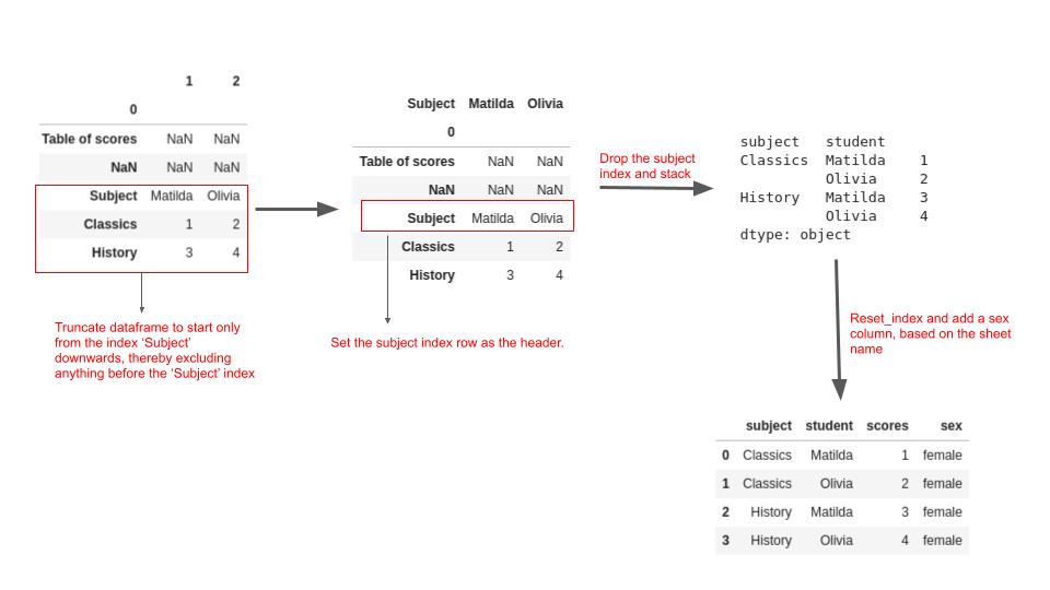
The image below explains the main concepts of the solution above :

Case 4 : Implied multiples

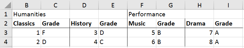
For this case, we have the fields at the top, followed by the subjects and grade for each subject. the student names is the very first column.
The goal is to get the subjects,grades and scores per field, per student and combine into one.

(excel_file
.parse(sheet_name='implied-multiples', header=None)
.ffill(axis=1)
.replace({np.nan : 'field'})
.set_index(0)
.T
.melt(id_vars = ['field','Name'],
      var_name = 'student',
      value_name = 'scores'
)
.assign(grade = lambda x: x.loc[x.Name == "Grade", 'scores'])
#scores are above grades per student
#hence the bfill
.bfill()
.query('Name != "Grade"')
.rename(columns={'Name':'subject'})
)

	field	subject	student	scores	grade
0	Humanities	Classics	Matilda	1	F
2	Humanities	History	Matilda	3	D
4	Performance	Music	Matilda	5	B
6	Performance	Drama	Matilda	7	A
8	Humanities	Classics	Olivia	2	D
10	Humanities	History	Olivia	4	C
12	Performance	Music	Olivia	6	B
14	Performance	Drama	Olivia	8	A

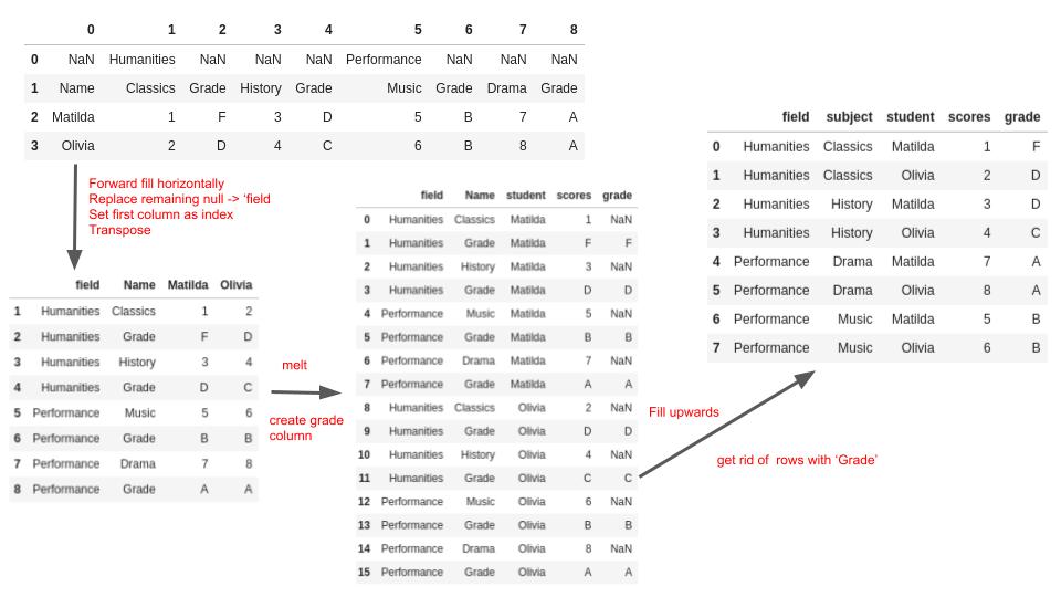
And a visual illustration of the steps is shown below: