Selecting and Grouping Data with Python Datatable

Datatable

This is a Python package for manipulating 2-dimensional tabular data structures (aka data frames). It is close in spirit to pandas or SFrame; however we put specific emphasis on speed and big data support. As the name suggests, the package is closely related to R’s data.table and attempts to mimic its core algorithms and API.

I like datatable primarily because of its simple syntax. Yes, there are significant speed gains, which is the primary aim of the package, but the simplicity is compelling.

Do note that datatable is in active development - more features will be added. Check out the documentation for more information.

This introduction focuses on how to select rows, select and perform calculations on columns, and perform aggregations by group.

Datatable syntax

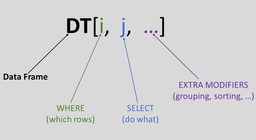
Short syntax right? Let’s break it down :
- DT refers to the data frame. This is the fundamental building block in datatable. It is a 2-dimensional array with rows and columns, similar to an Excel/SQL table.
- The i part is used for subsetting on rows and shares a similar concept with SQL’s WHERE clause.
- The j part is used to select columns and act on them.
- ... are for extra modifiers, e.g grouping, sorting, joining, etc.

Let’s dive into some examples to see how datatable works. Our data will be the iris dataset.

#import datatable
from datatable import dt, f, by

#read in data
DT = dt.fread("Data_files/iris.csv")

DT.head()

	sepal_length	sepal_width	petal_length	petal_width	species
	▪▪▪▪▪▪▪▪	▪▪▪▪▪▪▪▪	▪▪▪▪▪▪▪▪	▪▪▪▪▪▪▪▪	▪▪▪▪
0	5.1	3.5	1.4	0.2	setosa
1	4.9	3	1.4	0.2	setosa
2	4.7	3.2	1.3	0.2	setosa
3	4.6	3.1	1.5	0.2	setosa
4	5	3.6	1.4	0.2	setosa
5	5.4	3.9	1.7	0.4	setosa
6	4.6	3.4	1.4	0.3	setosa
7	5	3.4	1.5	0.2	setosa
8	4.4	2.9	1.4	0.2	setosa
9	4.9	3.1	1.5	0.1	setosa

10 rows × 5 columns

Notes :

• dt refers to the datatable module.

• All computations occur within the [] bracket.

• dt.fread is a powerful and very fast function for reading in various text files, zip archives, and urls. It can even read in data from the command line.

• by is a function for grouping.

• f is a variable that provides a convenient way to reference the data frame’s column within the square brackets. It is really useful when performing computations or creating expressions.

• In a jupyter notebook, the tab colours for the columns indicate various data types - blue is for float column, green is for integer column, red is for string column, yellow is for boolean, while black is for object column.

Some basic information about the data frame :

#shape of data
DT.shape

(150, 5)

#column names
DT.names

('sepal_length', 'sepal_width', 'petal_length', 'petal_width', 'species')

#data types of the columns
DT.stypes

(stype.float64, stype.float64, stype.float64, stype.float64, stype.str32)

The i part - Subset Rows

Select the first three rows

#We can use python's slicing syntax to get the rows. 
DT[:3, :]

	sepal_length	sepal_width	petal_length	petal_width	species
	▪▪▪▪▪▪▪▪	▪▪▪▪▪▪▪▪	▪▪▪▪▪▪▪▪	▪▪▪▪▪▪▪▪	▪▪▪▪
0	5.1	3.5	1.4	0.2	setosa
1	4.9	3	1.4	0.2	setosa
2	4.7	3.2	1.3	0.2	setosa

3 rows × 5 columns

Notes :

• No new syntax, just our knowledge of python’s sequence indexing.

• Note also that nothing was selected in the columns. Passing None or ... in the j section will work as well.

Select the 2nd, 4th and 8th rows

#Python has a zero based indexing notation,
#so, we will pass in a list [1,3,7]

DT[[1,3,7], :]

	sepal_length	sepal_width	petal_length	petal_width	species
	▪▪▪▪▪▪▪▪	▪▪▪▪▪▪▪▪	▪▪▪▪▪▪▪▪	▪▪▪▪▪▪▪▪	▪▪▪▪
0	4.9	3	1.4	0.2	setosa
1	4.6	3.1	1.5	0.2	setosa
2	5	3.4	1.5	0.2	setosa

3 rows × 5 columns

Find rows where species == “versicolor”

This is an expression. How do we talk to the dataframe to filter for only rows where the species column is equal to versicolor? Through the f variable :

result = DT[f.species == "versicolor", :]
result.head()

	sepal_length	sepal_width	petal_length	petal_width	species
	▪▪▪▪▪▪▪▪	▪▪▪▪▪▪▪▪	▪▪▪▪▪▪▪▪	▪▪▪▪▪▪▪▪	▪▪▪▪
0	7	3.2	4.7	1.4	versicolor
1	6.4	3.2	4.5	1.5	versicolor
2	6.9	3.1	4.9	1.5	versicolor
3	5.5	2.3	4	1.3	versicolor
4	6.5	2.8	4.6	1.5	versicolor
5	5.7	2.8	4.5	1.3	versicolor
6	6.3	3.3	4.7	1.6	versicolor
7	4.9	2.4	3.3	1	versicolor
8	6.6	2.9	4.6	1.3	versicolor
9	5.2	2.7	3.9	1.4	versicolor

10 rows × 5 columns

Notes :

• We create a boolean expression, using the f symbol, to select rows that match the condition.

Find rows where species == “versicolor” and sepal_length == 7

DT[(f.species == "versicolor") & (f.sepal_length == 7), :]

	sepal_length	sepal_width	petal_length	petal_width	species
	▪▪▪▪▪▪▪▪	▪▪▪▪▪▪▪▪	▪▪▪▪▪▪▪▪	▪▪▪▪▪▪▪▪	▪▪▪▪
0	7	3.2	4.7	1.4	versicolor

1 row × 5 columns

Notes :

• Again, a filter expression is needed -> we use the f symbol to access the columns and create our expression.

• Note also that we have two conditions; as such, each condition is wrapped in parentheses to ensure the operator precedence.

• Operator & for and, | for or.

• You can chain as many conditions as needed within the i section.

The j part - Columns

Select species, petal_width and petal_length columns

#Simply pass a list of the names in the j section 
result = DT[:, ["species","petal_width","petal_length"]]

result.head()

	species	petal_width	petal_length
	▪▪▪▪	▪▪▪▪▪▪▪▪	▪▪▪▪▪▪▪▪
0	setosa	0.2	1.4
1	setosa	0.2	1.4
2	setosa	0.2	1.3
3	setosa	0.2	1.5
4	setosa	0.2	1.4
5	setosa	0.4	1.7
6	setosa	0.3	1.4
7	setosa	0.2	1.5
8	setosa	0.2	1.4
9	setosa	0.1	1.5

10 rows × 3 columns

Notes :

• Note that we passed : in the i section to indicate that all rows will be selected. None or ... works fine as well.

Select the last two columns

#Again, we use python's indexing syntax
result = DT[:, -2:]

result.head()

	petal_width	species
	▪▪▪▪▪▪▪▪	▪▪▪▪
0	0.2	setosa
1	0.2	setosa
2	0.2	setosa
3	0.2	setosa
4	0.2	setosa
5	0.4	setosa
6	0.3	setosa
7	0.2	setosa
8	0.2	setosa
9	0.1	setosa

10 rows × 2 columns

Select only columns whose names end with length

result = DT[:, [col.endswith("length") for col in DT.names]]

result.head()

	sepal_length	petal_length
	▪▪▪▪▪▪▪▪	▪▪▪▪▪▪▪▪
0	5.1	1.4
1	4.9	1.4
2	4.7	1.3
3	4.6	1.5
4	5	1.4
5	5.4	1.7
6	4.6	1.4
7	5	1.5
8	4.4	1.4
9	4.9	1.5

10 rows × 2 columns

Notes:

• For this, we pass a list comprehension to extract the matches. Again, we are using familar python constructs.

Calculate the mean value of sepal_length

DT[:, f.sepal_length.mean()]

	sepal_length
	▪▪▪▪▪▪▪▪
0	5.84333

1 row × 1 column

• Here, we have to compute a value, and as such, the f symbol comes into play.

• To get the average, we use the mean function from the datatable module.

REMEMBER: Any time you want to compute a value or create an expression, make use of the f symbol.

TIP : We can export the column names and use them, instead of the f symbol :

sepal_length,  *_ = DT.export_names()

#calculate the mean value of sepal_length
DT[:, sepal_length.mean()]

	sepal_length
	▪▪▪▪▪▪▪▪
0	5.84333

1 row × 1 column

We can also export only the names we need :

petal_width, petal_length = DT[:, [2,3]].export_names()

#calculate mean value of petal_width and petal_length
DT[:, dt.mean([petal_width.mean(), petal_length])]

	petal_length	petal_width
	▪▪▪▪▪▪▪▪	▪▪▪▪▪▪▪▪
0	3.758	1.19933

1 row × 2 columns

Notes:

• To get aggregates of more than one column, pass a list of column names prefixed with the f symbol to j.

• Alternatively, you can pass a dictionary of key - value pairs, where the keys will be the new column names, and the values are the computed columns.

For the rest of the tutorial, I will continue using f-expressions, as they are convenient to use, without having to explicitly export column names.

Select only species and petal_length columns for rows where the petal_length is greater than 1.5

result = DT[f.petal_length > 1.5, ["species", "petal_length"]]

result.head()

	species	petal_length
	▪▪▪▪	▪▪▪▪▪▪▪▪
0	setosa	1.7
1	setosa	1.6
2	setosa	1.7
3	setosa	1.7
4	setosa	1.7
5	setosa	1.9
6	setosa	1.6
7	setosa	1.6
8	setosa	1.6
9	setosa	1.6

10 rows × 2 columns

Select only string columns

result = DT[:, f[str]]
result.head()

	species
	▪▪▪▪
0	setosa
1	setosa
2	setosa
3	setosa
4	setosa
5	setosa
6	setosa
7	setosa
8	setosa
9	setosa

10 rows × 1 column

Notes:

• The above concept is applicable for any data type that we wish to include or exclude from the dataframe

Convert petal_length from float to integer

• Option 1. Direct assignment :

result = DT.copy()

result["petal_length"].stype

stype.float64

#change column type
result["petal_length"] = dt.int32

#check new data type
result[:, f.petal_length].stype

stype.int32

• Option 2. Use the update method. The process is done in-place; no assignment is needed :

res = DT.copy()

res["petal_length"].stype

stype.float64

#update is an inplace operation
res[:, dt.update(petal_length = dt.int32(f.petal_length))]

#check data type after update 
res['petal_length'].stype

stype.int32

• Option 3. Use the as_type method. This is the recommended way to change the column type.

DT[:, f.petal_length.as_type(dt.int32)].stype

stype.int32

TIP : The update method allows creation of new columns, or updating existing ones.

Multiply petal_length by 2 and add it as a new column petal_double

• Option 1. Direct Assignment :

sol_1 = DT.copy()

sol_1["petal_double"] = sol_1[:, 2 * f.petal_length]

sol_1.head(5)

	sepal_length	sepal_width	petal_length	petal_width	species	petal_double
	▪▪▪▪▪▪▪▪	▪▪▪▪▪▪▪▪	▪▪▪▪▪▪▪▪	▪▪▪▪▪▪▪▪	▪▪▪▪	▪▪▪▪▪▪▪▪
0	5.1	3.5	1.4	0.2	setosa	2.8
1	4.9	3	1.4	0.2	setosa	2.8
2	4.7	3.2	1.3	0.2	setosa	2.6
3	4.6	3.1	1.5	0.2	setosa	3
4	5	3.6	1.4	0.2	setosa	2.8

5 rows × 6 columns

• Option 2. Use the extend method and pass in a dictionary of key value pairs, where the key is the new column name, and the value is the computed column:

sol_2 = DT.copy()

#f[:] means the entire columns are selected
sol_2 = sol_2[:, f[:].extend({"petal_double" : 2 * f.petal_length})]

sol_2.head(5)

	sepal_length	sepal_width	petal_length	petal_width	species	petal_double
	▪▪▪▪▪▪▪▪	▪▪▪▪▪▪▪▪	▪▪▪▪▪▪▪▪	▪▪▪▪▪▪▪▪	▪▪▪▪	▪▪▪▪▪▪▪▪
0	5.1	3.5	1.4	0.2	setosa	2.8
1	4.9	3	1.4	0.2	setosa	2.8
2	4.7	3.2	1.3	0.2	setosa	2.6
3	4.6	3.1	1.5	0.2	setosa	3
4	5	3.6	1.4	0.2	setosa	2.8

5 rows × 6 columns

• Option 3. The update method :

sol_3 = DT.copy()

sol_3[:, dt.update(petal_double = 2 * f.petal_length)]

sol_3.head(5)

	sepal_length	sepal_width	petal_length	petal_width	species	petal_double
	▪▪▪▪▪▪▪▪	▪▪▪▪▪▪▪▪	▪▪▪▪▪▪▪▪	▪▪▪▪▪▪▪▪	▪▪▪▪	▪▪▪▪▪▪▪▪
0	5.1	3.5	1.4	0.2	setosa	2.8
1	4.9	3	1.4	0.2	setosa	2.8
2	4.7	3.2	1.3	0.2	setosa	2.6
3	4.6	3.1	1.5	0.2	setosa	3
4	5	3.6	1.4	0.2	setosa	2.8

5 rows × 6 columns

• Option 4. Use the alias method:

DT[:, [f[:], (f.petal_length*2).alias('petal_double')]]

	sepal_length	sepal_width	petal_length	petal_width	species	petal_double
	▪▪▪▪▪▪▪▪	▪▪▪▪▪▪▪▪	▪▪▪▪▪▪▪▪	▪▪▪▪▪▪▪▪	▪▪▪▪	▪▪▪▪▪▪▪▪
0	5.1	3.5	1.4	0.2	setosa	2.8
1	4.9	3	1.4	0.2	setosa	2.8
2	4.7	3.2	1.3	0.2	setosa	2.6
3	4.6	3.1	1.5	0.2	setosa	3
4	5	3.6	1.4	0.2	setosa	2.8
5	5.4	3.9	1.7	0.4	setosa	3.4
6	4.6	3.4	1.4	0.3	setosa	2.8
7	5	3.4	1.5	0.2	setosa	3
8	4.4	2.9	1.4	0.2	setosa	2.8
9	4.9	3.1	1.5	0.1	setosa	3
10	5.4	3.7	1.5	0.2	setosa	3
11	4.8	3.4	1.6	0.2	setosa	3.2
12	4.8	3	1.4	0.1	setosa	2.8
13	4.3	3	1.1	0.1	setosa	2.2
14	5.8	4	1.2	0.2	setosa	2.4
⋮	⋮	⋮	⋮	⋮	⋮	⋮
145	6.7	3	5.2	2.3	virginica	10.4
146	6.3	2.5	5	1.9	virginica	10
147	6.5	3	5.2	2	virginica	10.4
148	6.2	3.4	5.4	2.3	virginica	10.8
149	5.9	3	5.1	1.8	virginica	10.2

150 rows × 6 columns

Drop the sepal_width column from the table

• Option 1. Use the del keyword :

del sol_1["sepal_width"]

sol_1.names

('sepal_length', 'petal_length', 'petal_width', 'species', 'petal_double')

sol_1.head(3)

	sepal_length	petal_length	petal_width	species	petal_double
	▪▪▪▪▪▪▪▪	▪▪▪▪▪▪▪▪	▪▪▪▪▪▪▪▪	▪▪▪▪	▪▪▪▪▪▪▪▪
0	5.1	1.4	0.2	setosa	2.8
1	4.9	1.4	0.2	setosa	2.8
2	4.7	1.3	0.2	setosa	2.6

3 rows × 5 columns

Option 2. Use the remove method :

sol_3 = sol_3[:, f[:].remove(f.sepal_width)]
sol_3.names

('sepal_length', 'petal_length', 'petal_width', 'species', 'petal_double')

sol_3.head(3)

	sepal_length	petal_length	petal_width	species	petal_double
	▪▪▪▪▪▪▪▪	▪▪▪▪▪▪▪▪	▪▪▪▪▪▪▪▪	▪▪▪▪	▪▪▪▪▪▪▪▪
0	5.1	1.4	0.2	setosa	2.8
1	4.9	1.4	0.2	setosa	2.8
2	4.7	1.3	0.2	setosa	2.6

3 rows × 5 columns

• Option 3. Use a list comprehension

DT[:, [name!='sepal_width' for name in DT.names]]

	sepal_length	petal_length	petal_width	species
	▪▪▪▪▪▪▪▪	▪▪▪▪▪▪▪▪	▪▪▪▪▪▪▪▪	▪▪▪▪
0	5.1	1.4	0.2	setosa
1	4.9	1.4	0.2	setosa
2	4.7	1.3	0.2	setosa
3	4.6	1.5	0.2	setosa
4	5	1.4	0.2	setosa
5	5.4	1.7	0.4	setosa
6	4.6	1.4	0.3	setosa
7	5	1.5	0.2	setosa
8	4.4	1.4	0.2	setosa
9	4.9	1.5	0.1	setosa
10	5.4	1.5	0.2	setosa
11	4.8	1.6	0.2	setosa
12	4.8	1.4	0.1	setosa
13	4.3	1.1	0.1	setosa
14	5.8	1.2	0.2	setosa
⋮	⋮	⋮	⋮	⋮
145	6.7	5.2	2.3	virginica
146	6.3	5	1.9	virginica
147	6.5	5.2	2	virginica
148	6.2	5.4	2.3	virginica
149	5.9	5.1	1.8	virginica

150 rows × 4 columns

Extra Modifiers

Notes :

• We will focus on grouping and sorting.

Sort data by sepal_width

outcome = DT[:, :, dt.sort('sepal_width')]

outcome.head()

	sepal_length	sepal_width	petal_length	petal_width	species
	▪▪▪▪▪▪▪▪	▪▪▪▪▪▪▪▪	▪▪▪▪▪▪▪▪	▪▪▪▪▪▪▪▪	▪▪▪▪
0	5	2	3.5	1	versicolor
1	6	2.2	4	1	versicolor
2	6.2	2.2	4.5	1.5	versicolor
3	6	2.2	5	1.5	virginica
4	4.5	2.3	1.3	0.3	setosa
5	5.5	2.3	4	1.3	versicolor
6	6.3	2.3	4.4	1.3	versicolor
7	5	2.3	3.3	1	versicolor
8	4.9	2.4	3.3	1	versicolor
9	5.5	2.4	3.8	1.1	versicolor

10 rows × 5 columns

• That’s all there is to it, just pass in the column name, either as a string or as an f expression.

• By default, sorting is in ascending order.

Sort by sepal_width ascending and petal_width descending

outcome = DT[:, :, dt.sort([f.sepal_width, -f.petal_width])]

outcome.head()

	sepal_length	sepal_width	petal_length	petal_width	species
	▪▪▪▪▪▪▪▪	▪▪▪▪▪▪▪▪	▪▪▪▪▪▪▪▪	▪▪▪▪▪▪▪▪	▪▪▪▪
0	5	2	3.5	1	versicolor
1	6.2	2.2	4.5	1.5	versicolor
2	6	2.2	5	1.5	virginica
3	6	2.2	4	1	versicolor
4	5.5	2.3	4	1.3	versicolor
5	6.3	2.3	4.4	1.3	versicolor
6	5	2.3	3.3	1	versicolor
7	4.5	2.3	1.3	0.3	setosa
8	5.5	2.4	3.8	1.1	versicolor
9	4.9	2.4	3.3	1	versicolor

10 rows × 5 columns

Notes :

• When sorting on multiple columns, pass a list of the column names to the sort function.

• The - sign in front of petal_width instructs data table to sort in descending order. The - is symbolic and no actual negation occurs; as such it can be used on string columns.

• Note that at this point, we had to switch to f-expression to get the desired result.

Group By - Get the average sepal length per species

DT[:, f.sepal_length.mean(), by("species")] 

	species	sepal_length
	▪▪▪▪	▪▪▪▪▪▪▪▪
0	setosa	5.006
1	versicolor	5.936
2	virginica	6.588

3 rows × 2 columns

Notes :

• by is the primary way to group data in the datatable.

• Since we are computing a value (average), the f symbol is used.

Group By - Get the average sepal length and petal length per species

DT[:, dt.mean([f.sepal_length, f.petal_length]), by("species")]

	species	sepal_length	petal_length
	▪▪▪▪	▪▪▪▪▪▪▪▪	▪▪▪▪▪▪▪▪
0	setosa	5.006	1.462
1	versicolor	5.936	4.26
2	virginica	6.588	5.552

3 rows × 3 columns

Group By - Filter the rows for sepal_width greater than or equal to 3, then get the average sepal length and petal length per species

DT[f.sepal_width>=3,:][:,dt.mean([f.sepal_length, f.petal_length]), by("species")]

	species	sepal_length	petal_length
	▪▪▪▪	▪▪▪▪▪▪▪▪	▪▪▪▪▪▪▪▪
0	setosa	5.02917	1.46667
1	versicolor	6.21875	4.54375
2	virginica	6.76897	5.64138

3 rows × 3 columns

Notes :

• At the moment, computation on i, j and by at the same time is not yet implemented. As such, we have to break down the steps into two parts.

• This also shows the chaining capabilities of datatable; simply put the next [], and datatable will compute the results from left to right.

Group By - Get the average sepal length and group on sepal width greater than 3

DT[:, dt.mean(f.sepal_length), by((f.sepal_width > 3).alias('sepal_width_gt_3'))]

	sepal_width_gt_3	sepal_length
	▪	▪▪▪▪▪▪▪▪
0	0	5.97229
1	1	5.68358

2 rows × 2 columns

Notes :

• With by, you can group on boolean expressions. Note the use of f-expression in the by function.

• Integers 0 and 1 signifiy False and True respectively.

Group By - Get the count of each species, and label the aggregation column as species_count

DT[:, {"species_count" : dt.count()}, by("species")]

	species	species_count
	▪▪▪▪	▪▪▪▪▪▪▪▪
0	setosa	50
1	versicolor	50
2	virginica	50

3 rows × 2 columns

Notes :

• As with previous examples, a column can be renamed by passing a dictionary, where the key is the new column name and the value is the aggregation result.

• count is another aggregation function within datatable.

Group By - Get the count of each species where the sepal width is greater than 3

DT[:, dt.count(), by(f.species, (f.sepal_width > 3).alias('sepal_width_gt_3'))]

	species	sepal_width_gt_3	count
	▪▪▪▪	▪	▪▪▪▪▪▪▪▪
0	setosa	0	8
1	setosa	1	42
2	versicolor	0	42
3	versicolor	1	8
4	virginica	0	33
5	virginica	1	17

6 rows × 3 columns

Notes :

• The by function can take a combination of columns, including booleans.

Summary

This was an introduction to the syntax of python datatable. We will explore more features in subsequent blog posts.